User Guide

Importing Alphafold Data

Supported formats

The af_analysis package supports the following file formats for input data:

• Alphafold 2 [1] and 3 [2]

• ColabFold [3]

• AlphaPulldown [4]

Importing procedure

Create the Data object, giving the path of the directory containing the results of the AlphaFold results. af_analysis supports reading the following directory formats:

• Alphafold 2 [1]

• Alphafold 3 [2]

• ColabFold [3]

• AlphaPulldown [4]

• Chai-1 [5]

• Boltz1 [6]

• MassiveFold [12]

import af_analysis
my_data = af_analysis.Data('MY_AF_RESULTS_DIR')

For AlphaPulldown and MassiveFold, you should explicitly define the format when importing the data:

import af_analysis
my_data = af_analysis.Data('MY_AF_RESULTS_DIR', format="alphapulldown")
# or
my_data = af_analysis.Data("MY_AF_RESULTS_DIR", format="massivefold")

Alternatively, you can use a python dictionary containing the pdb file list, the .json / .npz data file and the query name.

import af_analysis

pdb_list = [
    "test/model_5_seed_002.pdb",
    "test/model_5_seed_007.pdb",
    "test/model_5_seed_003.pdb",
    "test/model_5_seed_006.pdb",
    "test/model_5_seed_004.pdb",
]
json_list = [
    "test/model_5_seed_002.json",
    "test/model_5_seed_007.json",
    "test/model_5_seed_003.json",
    "test/model_5_seed_006.json",
    "test/model_5_seed_004.json",
]
data_dict = {
    "data_file": json_list,
    "pdb": pdb_list,
    "query": "test_amyloid",
}

my_data = af_analysis.Data(data_dict=data_dict)
# Extract the data that you know are present in the json/pickle files
my_data.extract_fields(["plddt", "ptm", "iptm"])

Extracted data are available in the df attribute of the Data object as a pandas dataframe.

my_data.df

Merge Data objects

You can merge multiple Data objects into a single object using the concat_data() function.

my_data1 = af_analysis.Data('MY_AF_RESULTS_DIR1')
my_data2 = af_analysis.Data('MY_AF_RESULTS_DIR2')
my_data = af_analysis.concat_data([my_data1, my_data2])

Scores

pDockq

pDockQ (Predicted DockQ) [7] is a metric that predicts the quality of protein-protein interactions in dimer models. It uses a sigmoid function that considers the number of contacts in the interface (\(log(number \: of \: interface \: contacts)\)) and the average pLDDT (predicted lDDT score) of the interface residues (\(\overline{plDDT_{interface}}\)).

Implementation was inspired from https://gitlab.com/ElofssonLab/FoldDock/-/blob/main/src/pdockq.py.

The pdockq() function calculates the pDockq [7] score for each model in the dataframe. The pDockq score ranges from 0 to 1, with higher scores indicating better model quality.

\[pDockQ = \frac{L}{1 + e^{-k (x-x_{0})}} + b\]

where:

\[x = \overline{plDDT_{interface}} \cdot log(number \: of \: interface \: contacts)\]

\(L = 0.724\) is the maximum value of the sigmoid, \(k = 0.052\) is the slope of the sigmoid, \(x_{0} = 152.611\) is the midpoint of the sigmoid, and \(b = 0.018\) is the y-intercept of the sigmoid.

from af_analysis import analysis
analysis.pdockq(my_data)

For the multiple pDockQ or mpDockQ [8] this values are used: \(L = 0.728\), \(x0 = 309.375\), \(k = 0.098\) and \(b = 0.262\).

from af_analysis import analysis
analysis.mpdockq(my_data)

pDockq2

pDockQ2, or Predicted DockQ version 2 [9], is a metric used to estimate the quality of individual interfaces in multimeric protein complex models. Unlike the original pDockQ, pDockQ2 incorporates AlphaFold-Multimer’s Predicted Aligned Error (PAE) in its calculation, making it more sensitive to large, incorrect interfaces that might have high confidence scores based solely on interface size and pLDDT. pDockQ2 scores range from 0 to 1, with higher scores indicating better interface quality.

\[pDockQ_2 = \frac{L}{1 + exp [-k*(X_i-X_0)]} + b\]

with

\[X_i = \langle \frac{1}{1+(\frac{PAE_{int}}{d_0})^2} \rangle * \langle pLDDT \rangle_{int}\]

\(L = 1.31\) is the maximum value of the sigmoid, \(k = 0.075\) is the slope of the sigmoid, \(x_{0} = 84.733\) is the midpoint of the sigmoid, and \(b = 0.005\) is the y-intercept of the sigmoid.

Implementation was inspired from https://gitlab.com/ElofssonLab/afm-benchmark/-/blob/main/src/pdockq2.py.

from af_analysis import analysis
analysis.pdockq2(my_data)

LIS Score

The Local Interaction Score (LIS) [10] is a metric specifically designed to predict the likelihood of direct protein-protein interactions (PPIs) using output data from AlphaFold-Multimer [11]. Unlike metrics like interface pTM (ipTM), which measures the overall structural accuracy of a predicted complex, LIS focuses on areas within the predicted interface that have low Predicted Aligned Error (PAE) values. These low PAE values, often visualized as blue regions in AlphaFold output maps, represent areas of high confidence in the interaction prediction

Here’s how LIS is calculated:

• Local Interaction Areas (LIAs) are identified: Regions of the predicted interface with PAE values below a defined

  cutoff (typically 12 Å) are designated as LIAs.

• PAE values within LIAs are inverted and averaged: PAE values within LIAs are transformed to a 0-1 scale, with

  higher numbers indicating stronger interaction likelihood. These values are then averaged across the interface to produce the LIS score.

• The LIS method is particularly adept at detecting PPIs characterized by localized and flexible interactions, which

  may be missed by ipTM-based evaluations. This is particularly relevant for interactions involving intrinsically disordered regions (IDRs), which are often missed by structure-based metrics.

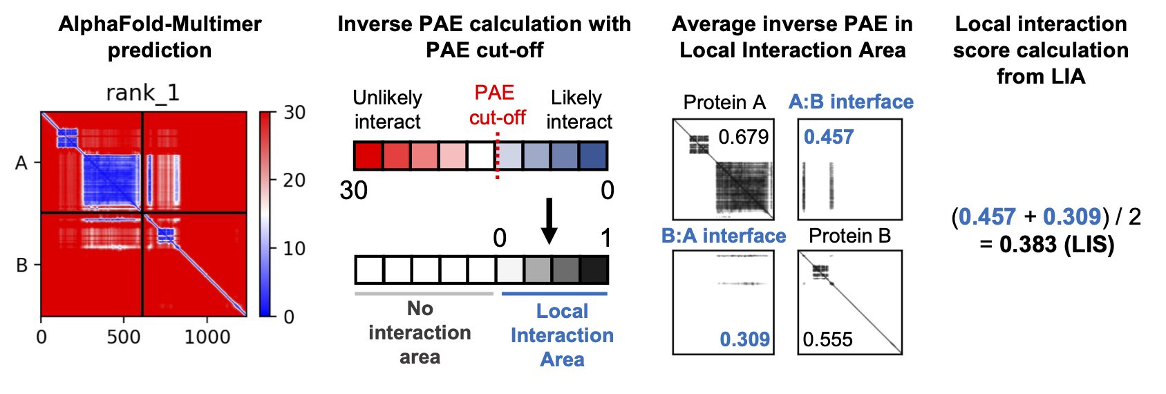
Figure from github.com/flyark/AFM-LIS. Implementation was inspired from https://github.com/flyark/AFM-LIS.

• to compute the LIS matrix among subunits:

from af_analysis import analysis
import seaborn as sns
from cmcrameri import cm

# Extract LIS heatmap among subunits
analysis.LIS_matrix(my_data, pae_cutoff=12.0)

# Plot the heatmap
ax = sns.heatmap(my_data.df.LIS.iloc[0], cmap=cm.roma)
ax.collections[0].set_clim(0,1)  # Set the heatmap range
ax.set_title('LIS heatmap among subunits')
ax.set_xlabel('Subunit index')
ax.set_ylabel('Subunit index')

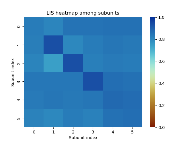
Example of LIS heatmap among subunits on a protein-DNA-Zn complex computed with AlphaFold 3.

actifpTM and chain ipTM

The actual interface pTM (actifpTM), has been included in colabfold version 1.5.5 (march 2025). If you have used the --calc-extra-ptm option to launch colabfold_batch command, the actifpTM and chain ipTM scores are available in the colabfold .json output files.

An extra step is necessary to extract the scores from the .json files:

my_data = af_analysis.Data('MY_AF_RESULTS_DIR')
my_data.extract_data()

You should now have access to additional columns in the dataframe:

my_data.df[['pairwise_actifptm', 'pairwise_iptm', 'per_chain_ptm', 'actifptm']]

• The pairwise_actifptm column contains the actifpTM scores for each pair of chains in the model.

• The pairwise_iptm column contains the ipTM scores for each pair of chains in the model.

• The per_chain_ptm column contains the pTM scores for each chain in the model.

• The actifptm column contains the actifpTM scores for each model in the dataframe.

Protein-Protein and Protein-Peptide Docking

The af_analysis package provides a simple interface to score protein-protein and protein-peptide docking using the docking package.

Note

The docking package infer that the peptide chain or the protein ligand chain is the last one in the model.

The docking package allow to compute:

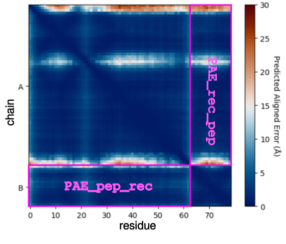
• pae_pep(): average interface of Predicted Aligned Error (PAE) between the receptor chain(s) and the

  ligand/peptide chain (last one). Add the columns PAE_pep_red and PAE_rec_pep in the dataframe.

• plddt_pep(): compute the average pLDDT of the ligand chain. Add the column plddt_pep in the dataframe.

• pdockq2_lig(): compute the pDockQ2 scores of each chain. Add the columns pdockq2_A, pdockq2_B, … and pdockq2_lig (the last chain pdockq2) in the dataframe.

• LIS_pep(): compute the Local Interaction Score (LIS) between the receptor chain(s) and the ligand/peptide chain (last one). Add the columns LIS_rec_pep and LIS_pep_rec in the dataframe.

Example:

from af_analysis import docking

#extract_pae_pep
docking.pae_pep(my_data)
#compute_pdockq2_lig
docking.pdockq2_lig(my_data)
#compute_LIS_pep
docking.LIS_pep(my_data)
#extract_plddt_pep
docking.plddt_pep(my_data)

Plots

Interactive Visualization

At first approach the user can visualize the pLDDT, PAE matrix and the model scores. The show_info() function displays the scores of the models, as well as the pLDDT plot and PAE matrix in a interactive way.

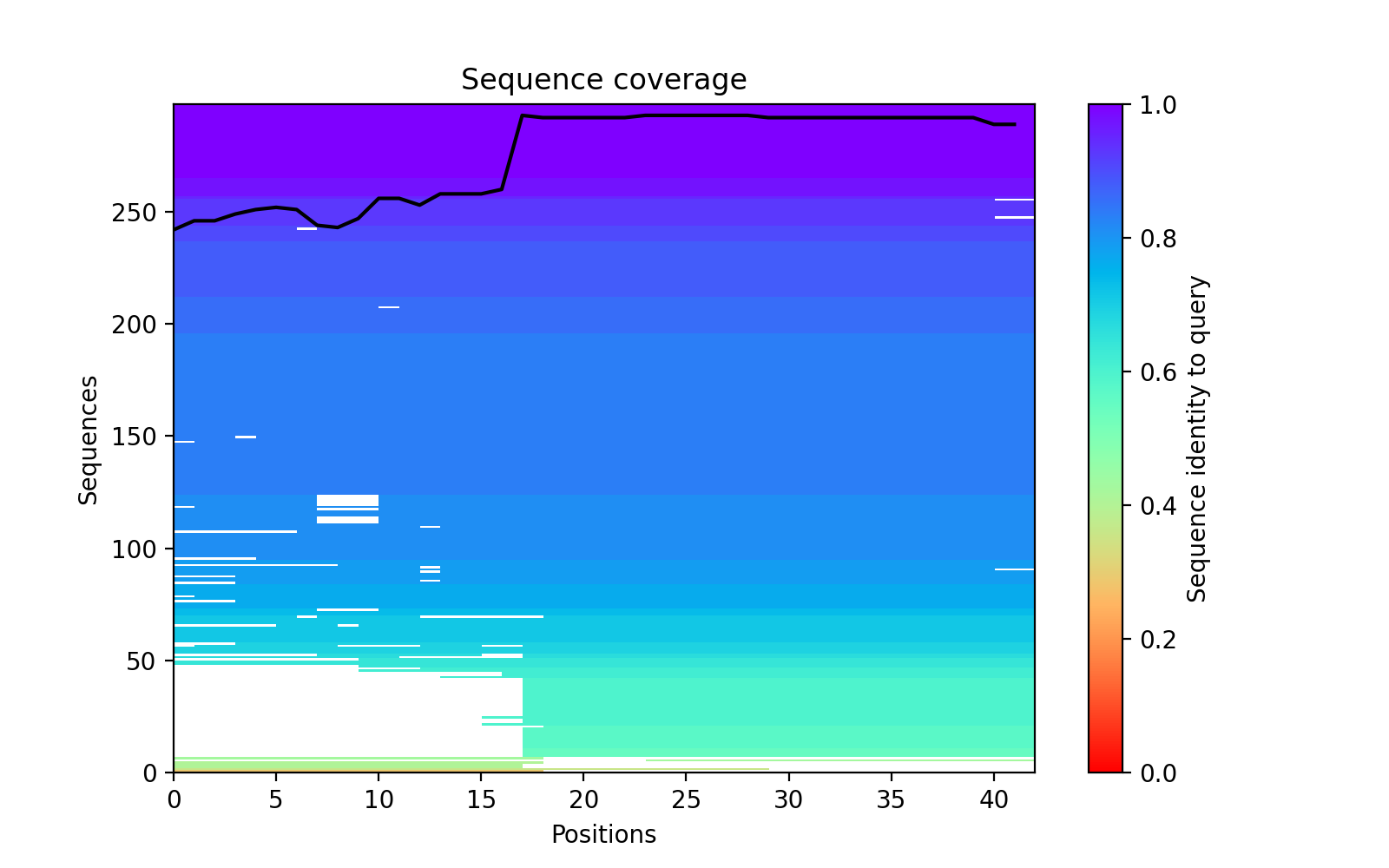
MSA Plot

The plot_msa() function generates a multiple sequence alignment (MSA) plot for the predicted models. The MSA plot shows the sequence conservation of the predicted models, highlighting regions of high and low conservation.

my_data.plot_msa()

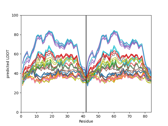
pLDDT Plot

The plot_plddt() function generates a pLDDT plot for the predicted models. The pLDDT plot shows the per-residue local distance difference test (pLDDT) score for each residue in the predicted models, highlighting regions of high and low model confidence.

• you can plot all models plddt at once:

my_data.plot_plddt()

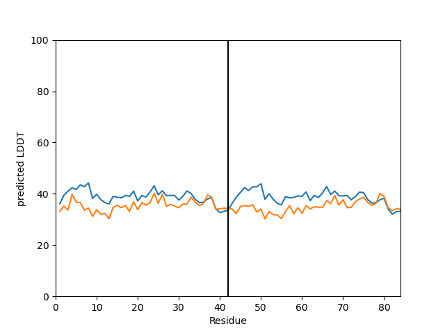
• or you can plot specific models plddt:

my_data.plot_plddt([0,1])

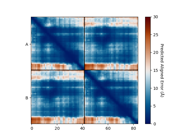
PAE Plot

The plot_pae() function generates a predicted aligned error (PAE) plot for the predicted models. The PAE plot shows the per-residue predicted aligned error for each residue in the predicted models, highlighting regions of high and low model accuracy.

best_model_index = my_data.df['ranking_confidence'].idxmax()
my_data.plot_pae(best_model_index)

3D Structure Visualization

The show_3d() function displays the 3D structure of the predicted models using the nglview package. The 3D structure visualization allows users to interactively explore the predicted models and compare them with the experimental structure.

my_data.show_3d(my_data.df['ranking_confidence'].idxmax())

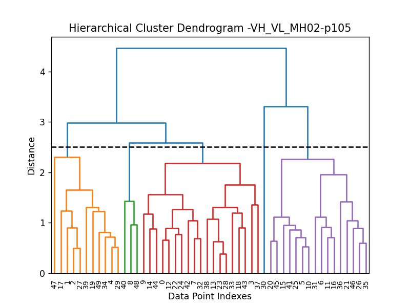
Clustering

This approach aims to address the challenge of managing and analyzing the large number of models (e.g., 10.000) produced for each protein complex, especially since these models often exhibit structural redundancies.

To do so, the user can use the clustering module to cluster the models based on their structural similarity. The user can choose:

• a selection to align model structures, e.g. "backbone and chain A"

• a selection to calculate the RMSD matrices, e.g. , "backbone and chain B",

• a threshold value to determine the number of clusters.

• RMSD can be scaled using Björn Wallner method:

\[RMS_{scaled} (RMS, di) = \frac{1}{1 + (\frac{RMS}{di})^2}\]

with \(RMS\) the RMSD matrix and \(di\) a scaling factor of 8.5 Å.

From the distance matrix (scaled or not), an ascending hierarchical classification is computed to determine the clusters based on the distance threshold.

from af_analysis import clustering

clustering.hierarchical(my_data.df, threshold=2.5)

A multidimensional scaling (MDS) coordinates can be computed from the distance matrix to visualize a 2D projection of the clusters, this coordinates are added in the dataframe in column MDS 1 and MDS 2.

sns.scatterplot(data=my_data.df, x='MDS 1', y='MDS 2', hue='cluster')

Custom Analysis functions

The user can define custom analysis functions to compute additional metrics or visualizations. In this example we use the pdb_cpp package to define the contact_number() function which take a pdb file as input and compute the number of contacts between chains.

# Here we use the `pdb_cpp` package to deal with coordinates file
import pdb_cpp

def contact_number(pdb, cutoff=8.0):
    # Compute the number of contacts in the interface
    coor = pdb_cpp.Coor(pdb)
    chains = np.unique(coor.chain)
    contact_num = 0

    for chain in chains:
        coor_interface = coor.select_atoms(
            f"name CA and chain {chain} and within {cutoff} of not chain {chain}")
        contact_num += coor_interface.len

    return contact_num

The custom analysis function can then be applied easily to the dataframe:

# Apply the custom analysis function to the dataframe
contact_list = []
for pdb in my_data.df.pdb:
    contact_list.append(contact_number(pdb))
# Add the contact number to the dataframe
my_data.df['contact_num'] = contact_list

The custom analysis results are then stored in the dataframe as the contact_num column and can be used for further analysis.

FTDMP Scores

The af_analysis package provides a simple interface to extract docking score computed using the FTDMP software.

First you need to install the ftdmp package:

git clone https://github.com/kliment-olechnovic/ftdmp.git
cd ./ftdmp
./core/build.bash

• and then install dependencies using conda:

conda env create -f ftdmp_environment_for_conda.yml

Then you can use the FTDMP sofware to compute different scores from the pdb files:

conda activate ftdmp
ls MY_AF_DIRECTORY/*.pdb | ~/Documents/Code/ftdmp/ftdmp-qa-all --workdir ftdmp_beta_amyloid_dimer

you can then extract the scores using the analysis.extract_ftdmp() function in a python script or a jupyter notebook :

import af_analysis
from af_analysis import analysis

my_data = af_analysis.Data('MY_AF_RESULTS_DIR')
# Extract the FTDMP scores
analysis.extract_ftdmp(my_data, ftdmp_path='ftdmp_beta_amyloid_dimer')

If you use the FTDMP software, please cite:

• Olechnovič K, Banciul R, Dapkūnas J, Venclovas Č. (2025) FTDMP: A Framework for Protein-Protein, Protein-DNA, and Protein-RNA Docking and Scoring. Proteins. doi: 10.1002/prot.26792. PubMed PMID: 39748638.

Scoring of protein-protein interfaces using the VoroIF-jury algorithm and details of this algorithm are published in the CASP16 article:

• Olechnovič K, Valančauskas L, Dapkūnas J, Venclovas Č. (2023) Prediction of protein assemblies by structure sampling followed by interface-focused scoring. Proteins; 91:1724–1733. doi: 10.1002/prot.26569. PubMed PMID: 37578163.

Citing this work

If you use the code of this package, please cite:

• Reguei A and Murail S. Af-analysis: a Python package for Alphafold analysis.

  Journal of Open Source Software (2025) doi: 10.21105/joss.07577

@Article{reguei_af-analysis_2025,
    title = {Af-analysis: a {Python} package for {Alphafold} analysis},
    volume = {10},
    issn = {2475-9066},
    shorttitle = {Af-analysis},
    url = {https://joss.theoj.org/papers/10.21105/joss.07577},
    doi = {10.21105/joss.07577},
    language = {en},
    number = {107},
    urldate = {2025-03-14},
    journal = {Journal of Open Source Software},
    author = {Reguei, Alaa and Murail, Samuel},
    month = mar,
    year = {2025},
    pages = {7577},
}

References

[1] (1,2)

Jumper et al. Nature (2021) doi: 10.1038/s41586-021-03819-2

[2] (1,2)

Abramson et al. Nature (2024) doi: 10.1038/s41586-024-07487-w

[3] (1,2)

Mirdita et al. Nat Methods (2022) doi: 10.1038/s41592-022-01488-1

[4] (1,2)

Yu et al. Bioinformatics (2023) doi: 10.1093/bioinformatics/btac749

[5]

Chai Discovery et al. bioRxiv (2024) doi: 10.1101/2024.10.10.615955v2

[6]

Wohlwend et al. bioRxiv (2024) doi: 10.1101/2024.11.19.624167

[7] (1,2)

Bryant et al. Nat Commun (2022) doi: 10.1038/s41467-022-28865-w

[8]

Bryant et al. Nat Commun (2022) doi: 10.1038/s41467-022-33729-4

[9]

Zhu et al. Bioinformatics (2023) doi: 10.1093/bioinformatics/btad424

[10]

Kim et al. bioRxiv (2024) doi: 10.1101/2024.02.19.580970

[11]

Evans et al. bioRxiv (2021) doi: 10.1101/2021.10.04.463034

[12]

Raouraoua et al. Nat Comput Sci (2024) doi: 10.1038/s43588-024-00714-4