Basic Example
Importing packages
You first need to import the af_analysis package:
[ ]:
DATA_PATH = '../../../tests/inputs/beta_amyloid_dimer_cf_1.5.5/'

%matplotlib inline
Importing Alphafold Data
To import your data, create a af_analysis.Data object by giving the path of Alphafold directorie:
[2]:
DATA_PATH = '../../../src/af_analysis/test/inputs/beta_amyloid_dimer_cf_1.5.5/'
my_data = af_analysis.Data(DATA_PATH)
You now have access to a pandas DataFrame containing all models:
[3]:
my_data.df.head(2)
[3]:
| query | seed | model | weight | recycle | pLDDT | pTM | ipTM | ranking_confidence | format | pdb | relaxed_pdb | json | |
|---|---|---|---|---|---|---|---|---|---|---|---|---|---|
| 0 | beta_amyloid_dimer_d2fa3_0 | 0 | 1 | alphafold2_multimer_v3 | 9 | 38.8 | 0.159 | 0.0812 | 0.09676 | colabfold_1.5 | ../../../src/af_analysis/test/inputs/beta_amyl... | None | ../../../src/af_analysis/test/inputs/beta_amyl... |
| 1 | beta_amyloid_dimer_d2fa3_0 | 0 | 2 | alphafold2_multimer_v3 | 16 | 35.2 | 0.130 | 0.0685 | 0.08080 | colabfold_1.5 | ../../../src/af_analysis/test/inputs/beta_amyl... | None | ../../../src/af_analysis/test/inputs/beta_amyl... |
For each query of the directorie, the chains IDs and chain length will be store in chains and chain_length properties of the Data object:
[4]:
my_data.chain_length
[4]:
{'beta_amyloid_dimer_d2fa3_0': [42, 42]}
[5]:
my_data.chains
[5]:
{'beta_amyloid_dimer_d2fa3_0': ['A', 'B']}
Analysing scores
You can then sort or extract your models based on the score you are interrested in:
pLDDT
pTM
ipTM
ranking_confidence
Here I am extracting the best ipTM model index:
[6]:
best_ipTM_index = my_data.df['ipTM'].idxmax()
worst_ipTM_index = my_data.df['ipTM'].idxmin()
You can get access to all its caracteristics:
[7]:
my_data.df.iloc[best_ipTM_index]
[7]:
query                                        beta_amyloid_dimer_d2fa3_0
seed                                                                  2
model                                                                 5
weight                                           alphafold2_multimer_v3
recycle                                                               9
pLDDT                                                              68.3
pTM                                                               0.628
ipTM                                                              0.604
ranking_confidence                                               0.6088
format                                                    colabfold_1.5
pdb                   ../../../src/af_analysis/test/inputs/beta_amyl...
relaxed_pdb           ../../../src/af_analysis/test/inputs/beta_amyl...
json                  ../../../src/af_analysis/test/inputs/beta_amyl...
Name: 14, dtype: object
Plots
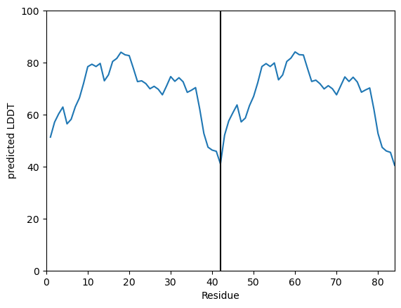
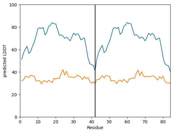
You can plot the the pLDDT for one model:
[8]:
my_data.plot_plddt([best_ipTM_index])
[8]:
(<Figure size 640x480 with 1 Axes>,
 <Axes: xlabel='Residue', ylabel='predicted LDDT'>)
[9]:
my_data.plot_plddt([best_ipTM_index, worst_ipTM_index])
[9]:
(<Figure size 640x480 with 1 Axes>,
 <Axes: xlabel='Residue', ylabel='predicted LDDT'>)
And also have a look on the Predicted Aligned Error (PAE) matrix:
[10]:
my_data.plot_pae(best_ipTM_index)
[10]:
(<Figure size 640x480 with 2 Axes>, <Axes: >)

show 3D structure
The 3D structure can be represented using the nglview library:
[11]:
view = my_data.show_3d(best_ipTM_index)
view
[14]:
IFrame(src='../_static/dimer.html', width=600, height=300)
[14]:
Computing scores
Additional scores can be computed as the pdockq and pdockq2:
[15]:
from af_analysis import analysis

#compute_pdockq
analysis.pdockq(my_data)
#compute_pdockq2
analysis.pdockq2(my_data)
Some additional scores have been compute to caracterise the protein-peptide structures:
[16]:
from af_analysis import docking

#extract_pae_pep
docking.pae_pep(my_data)
#compute_pdockq2_lig
docking.pdockq2_lig(my_data)
#compute_LIS_pep
docking.LIS_pep(my_data)
#extract_plddt_pep
docking.plddt_pep(my_data)
[17]:
my_data.df.columns
[17]:
Index(['query', 'seed', 'model', 'weight', 'recycle', 'pLDDT', 'pTM', 'ipTM',
       'ranking_confidence', 'format', 'pdb', 'relaxed_pdb', 'json', 'pdockq',
       'pdockq2_A', 'pdockq2_B', 'PAE_pep_rec', 'PAE_rec_pep', 'pdockq2_lig',
       'LIS', 'LIS_rec_pep', 'LIS_pep_rec', 'plddt_pep'],
      dtype='object')
Clustering
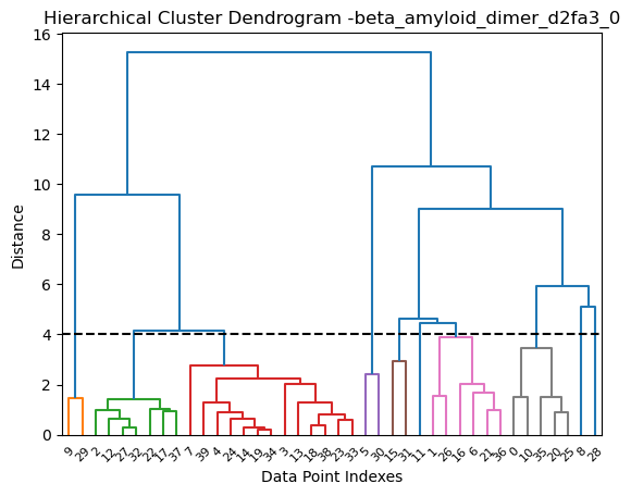
Eventually the obtain models can be clustered to have a better idea oh AlphaFold model diversity. Here we are using a thresold of 4 Å with hierarchical clustering:
[18]:
from af_analysis import clustering
clustering.hierarchical(my_data.df, threshold=4)
/home/murail/miniforge3/envs/SST2/lib/python3.12/site-packages/Bio/Application/__init__.py:39: BiopythonDeprecationWarning: The Bio.Application modules and modules relying on it have been deprecated.

Due to the on going maintenance burden of keeping command line application
wrappers up to date, we have decided to deprecate and eventually remove these
modules.

We instead now recommend building your command line and invoking it directly
with the subprocess module.
  warnings.warn(
/home/murail/miniforge3/envs/SST2/lib/python3.12/site-packages/MDAnalysis/coordinates/base.py:728: UserWarning: Reader has no dt information, set to 1.0 ps
  return self.ts.dt
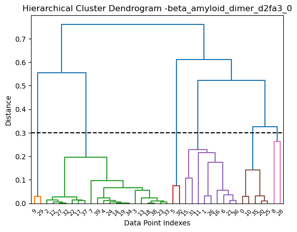
Alternatively, the RMSD can be normalized and scaled using Bjorn Wallner scaling. Here we are using a thresold of 0.3 with hierarchical clustering:
[19]:
clustering.hierarchical(my_data.df, threshold=0.3, rmsd_scale=True)
/home/murail/miniforge3/envs/SST2/lib/python3.12/site-packages/MDAnalysis/coordinates/base.py:728: UserWarning: Reader has no dt information, set to 1.0 ps
  return self.ts.dt
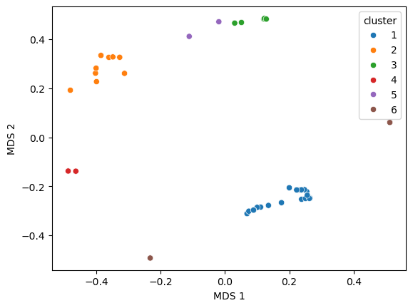
Multidimensional scaling representation
Multidimensional scaling (MDS) coordinates are computed from the distance matrix and added in the dataframe:
[20]:
import seaborn as sns
sns.scatterplot(data=my_data.df, x='MDS 1', y='MDS 2', hue='cluster')
[20]:
<Axes: xlabel='MDS 1', ylabel='MDS 2'>
[ ]: